
MOE home > Nature and Parks > EBSA home > Analysis used by scientific data
Analysis used by scientific data
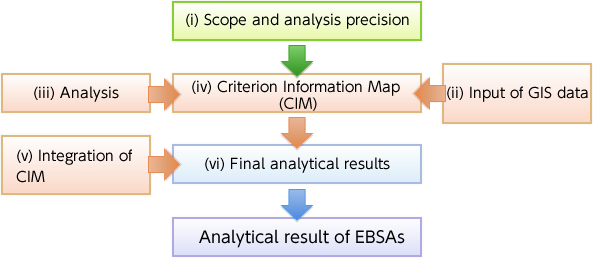
Identification of EBSAs was advanced mainly through the process shown in the diagram below. First, analysis precision (fineness of grids) and scopes were decided (more detail, see (i) scope and analysis precision). Then, data for practical use were identified for each criterion from the examples of applicationof each criterion in order to identify locations meeting those criteria, and a variety of data such as habitat and species distributions were input in GIS analysis (see (ii) Input of GIS data). Using GIS data, each grid was scored from 1 to 5 points to see the degree to which it met each criterion. To give a score in each grid, two analytical methods were carried out; the more data overlapped in a grid, the more highly scored, or the irreplaceable locations by complementary analysis were highly scored (see (iii) Analysis). Using this score, results of these analyses are firstly compiled as “Criterion Information Maps” (CIMs) (see (iv) Criterion Info. Map). CIMs needed to be integrated into one map to identify the EBSAs in coastal area, pelagic surface, and sea floor. Therefore, the same as when formulating CIM, the “highest scored grid,” where more data overlapped or where the area was evaluated as an irreplaceable grid by complementary analysis, were selected (see (v) Integration of Criterion Info. Map). As a result, final analytical result was formulated (see (vi) Final analytical results).
More detail of each of these steps, see (i)-(vi) described as below.
(i) Scope and analysis precision
In light of the fact that marine ecosystems need to be understood three-dimensionally (vertically and horizontally), we had taken that into in account. Accordingly, marine areas were divided into coastal areas (those in territorial waters up to 200 m deep), for which large quantities of data were available, and offshore areas. Then, the offshore areas were divided further into surface areas and sea floors for analysis; analysis was carried out in (i) coastal areas, (ii) offshore surface, (iii) offshore seafloor respectively. For coastal areas, a 5 km grid was employed (approx. 5 km square), while for offshore areas (both surface and sea floor), grids of 30 min (approx. 55 by 45 km, varying by latitude) were used as base units for GIS analysis.
(ii) Input of GIS data
Data available for use as GIS data were used as much as possible, including physical environmental data (e.g., sea floor topographical data, ocean currents), species and habitat distribution data (e.g., national survey of natural environment), official government data (e.g., important wetlands of Japan, Natural Monument), international agencies’ data (e.g., OBIS, GBIF, IBA, Marine-IBA), and other relevant data (e.g., WWF important coral reefs in Japan, key areas for conservation of insect diversity), as well as academic papers. These data were input for each criterion referring to the “examples of application” of each criterion. All of these various data formats (e.g., point data (longitude latitude), polygon data, and line data) were analyzed using 5 km grids for coastal areas (approx. 5 km square) and grids of 30 minutes (approx. 55 by 45 km) for offshore areas uniformly. In addition, since the data properties used in GIS analysis varied, they were grouped into the three categories: 1) distribution data of species, 2) habitat data of ecosystems such as coral reefs and seaweed beds, and 3) number of items such as natural monuments. Each of the three categories was analyzed separately.
(iii) Analysis
To prepare CIMs, showing which locations best satisfy each criterion, two analytical methods were employed. One of these assessed overlapping of species (or ecosystems), to identify locations where more factors (e.g., species and ecosystems) satisfying criteria overlapped. The other was a complementarity analysis that is the method of selecting most efficient grids for conservation with the minimum number of grids. For the complementarity analysis, MARXAN![]() (an algorithm for scientifically choosing high-priority sites for conservation of biodiversity and candidate sites for marine protected areas) was employed.
(an algorithm for scientifically choosing high-priority sites for conservation of biodiversity and candidate sites for marine protected areas) was employed.
Analytical methods other than those listed above were also used to see the degree of satisfaction depending on the criterion. For example, coverage of seaweed/seagrass beds or coral reefs in a grid for costal area, chlorophyll a density for pelagic surfaces was used for Criterion 5 to see the productivity. For Criterion 6 (biodiversity), Hurlbert’s Index was employed. For Criterion 7, coverage of natural coast and vegetation are used as well as overlapping of naturalness indicator species that only inhabit the place in high naturalness.
These methods were used to score each grid on a 1–5 scale.
(iv) Criterion Information Maps
The scores assigned in the process under (iii) were used to prepare the CIM. In the case of both analytical methods where overlapping and complementarity analysis each were used, a higher resulting score would be prioritized, so the results of the two analyses were integrated in assessing such grids.
In this way, formulation of CIM was conducted for each criterion in coastal areas, offshore surfaces, and offshore seafloor.
(v) Integration of Criterion Information Map
The CIM were integrated into a single map. Integration of CIMs was conducted through two methods using the scores assigned to each grid of the CIMs. Since the data volume of each criterion varied, complementarity analysis using MARXAN to identify high-priority grids across the eight criterion was employed (“high-priority grids”), while the highest score’s grids on each of the CIM were considered as important grids (“high-scoring grids”). Then the grids selected through these two methods were combined.
(vi) Analytical result of EBSAs
Each of the high-scoring grids and high-priority grids identified through the step (v) was selected as corresponding to EBSAs. Selected grids were united by the smoothing method of GIS automatically; then, these were charted as the analytical result of EBSAs.
![]()
Godochosha No. 5, Kasumigaseki 1-2-2, Chiyoda-ku, Tokyo 100-8975, Japan.
Tel: +81-(0)3-3581-3351